How To Get Values In Excel Pivot Table

To automatically fit the PivotTable columns to the size of the widest text or number value select the Autofit column widths on update check box. Youll see that Σ Values field in columns area.

Pivot Table Errors Pivot Table Excel Formula Pivot Table Excel

In the Name box select the calculated field for which you want to change the formula.

How to get values in excel pivot table. In this case we select cells B2F10. In the popup menu click Summarize Values By and then click Max. Just drag that in rows and you are done.

Try out Data Bars in Excel for clear graphical data representation. We do this by selecting our table then going to Insert. Choose Add This Data to the Data Model while creating the pivot table.

For our example we will use the table with NBA players their clubs the conference that their clubs are in and statistics from one or several matches. Once you click on Index you will get results as shown in the image below. Show Text in Pivot Values Area With Data Model.

To get a value from a pivot table in excel we use the function. We can count values in a PivotTable by using the value field settings. Merge Id Name Brand Model License inside the Helper column.

Be on any value cells. Insert a Pivot Table. To get what we want we have to make sure to add our data to the data model.

In the Create. On the Analyze tab in the Calculations group click Fields Items Sets and then click Calculated Field. Show values in a pivot table using VLOOKUP The first one uses a helper column with the VLOOKUP function.

Now when you start creating a pivot table. In the Value Field Settings dialog click Summarize Values By tab and then scroll to click Distinct Count option see screenshot. Make a note of the.

Copy pivot table and Paste SpecialValues to say L1. We want to get the sales for France from the pivot table. In the Formula box edit the formula.

Right click Show Values As Index. Drag Dates into Columns. Add the first field Sales into Values.

When using GETPIVOTDATA to fetch information from a pivot table based on a date or time date or time use Excels native format or a function like the DATE function. Create a new column called Helper between the Model and Licence columns. Heres how you can see the pivot table value settings.

Insert new cell at L1 and shift down. The pivot table values now show the correct region number for each value but instead of the numbers 1 2 or 3 wed like to see the name of the region East Central or West. How to Count Values in a Pivot Table.

In the above image you can see the value of each product in that particular region. The pivot table values changes to show the region numbers. Pivot Table With Text in Values Area Make sure your data is Formatted as Table by choosing one cell in the data and pressing Ctrl T.

This works well in a simple pivot table Jan 13 2021 Uploaded by Contextures Inc. Edit a calculated field formula. Inserting a Pivot Table.

For example to get total Sales on April 1 2021 when individual dates are displayed. To display the values in the rows of the pivot table follow the steps. To add a visual element to the pivot table add data bars that are similar to a bar chart.

OnNow i want to get the values from pivot tables as and when i select values corresponding to that values i need only the sum fields value. Click the Insert tab then Pivot Table. Delete top row of copied range with shift cells up.

For instance in the example below there is a count of 16 for clients when distinctly they are only 4. Now we will create our Pivot Table to derive the data that we need. This will launch the Create PivotTable dialog box.

This enables us to have a valid representation of what we have in our data. Select the range of cells that we want to analyze through a pivot table. Key Name into L1.

And then click OK you will get. Data_field this is the field in the pivot table that we want to retrieve in our example this is Sales. Change Region Numbers to Names.

This tutorial offers a step-by-step guide on how to add data bars in Excel. Imagine this simple data. In the PivotTable Options dialog box on the Layout Format tab under Format do one of the following.

Then add the second field Expenses into Values. Right-click a number in the Values area Point to Summarize Values By or Show Values As In the pop-up list the current setting has a check mark. Eg field namesA B Sum Values in filed A 123 Values in filed B 456 Values in field c 579 so wenever i select 1 in A 4 in B i should get the value of C5 in some empty cell of Excel.

To keep the current PivotTable column width clear the Autofit column widths on update check box.

Excel Pivot Tables Pivot Table Excel Pivot Table Excel

Show Monthly Values Changes In One Pivot Report Excel Pivot Table Examples Pivot Table Pivot Table Excel Excel

Multi Level Pivot Table In Excel Pivot Table Excel Excel Templates

Follow These Easy Steps To Create A Pivot Table In Microsoft Excel 2016 Excel Pivot Table Microsoft Excel Tutorial

Displaying Text Values In Pivot Tables Without Vba Pivot Table Text Excel

Excel Pivot Tables Pivot Table Data Science Excel

23 Things You Should Know About Pivot Tables Exceljet Pivot Table Excel Tips

Excel Pivot Tables Pivot Table Excel Shortcuts Excel

Excel Pivot Tables In 2021 Pivot Table Excel Tutorials Excel

Excel Pivot Tables Tutorial What Is A Pivot Table And How To Make One

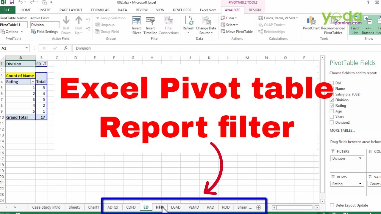
Excel Pivot Table Report Filter Advanced Excel Youtube Pivot Table Excel Tutorials Pivot Table Excel

How To Refresh All Values In Excel Pivot Tables In 2020 Pivot Table Pivot Table Excel Excel Tutorials

Setting Format Directly On A Value Field Pivot Table Excel Microsoft Excel

Create A Quick Access To Account Balances In Excel Balances Using Pivot Tables And Vlookup Create A Drop Down List With All The Excel Pivot Table Accounting

Get Correct Count In Excel Pivot Table Even With Blank Cells In Source Data Pivot Table Excel Workbook

Excel Pivot Tables Pivot Table Excel Fun Worksheets

Create The Pivot Table And Then Click Any Cell In The Pivot Table On Which You Want To Base The Chart In This Example The Data Is Found Pivot Table Excel

Pin On Pivot

How To Show Hide Field List In Excel Pivot Table Pivot Table Excel Tutorials Excel